Metagenomics tutorial part 1: Quality control, assembly and mapping
By Adam Rivers
Overview
Shotgun metagenomics data can be analyzed using several different approaches. Each approach is best suited for a particular group of questions. The methodological approaches can be broken down into three broad areas: read-based approaches, assembly-based approaches and detection-based approaches. This tutorial takes an assembly-based approach. The key points of the approaches are listed in this table:
| Method | Read-based | Assembly-based | Detection-based |
|---|---|---|---|
| Description | Read-based metagenomics analyzes unassembled reads. It was one of the first methods to be used. It is still valuable for quantitative analysis, especially if relevant references are available. | Assembly-based workflows attempt to assemble the reads from one or more samples, “bin” contigs from these samples into genomes then analyze the genes and contigs. | Detection-based workflows attempt to identify with very high-precision but lower sensitivity (recall) the presence of organisms of interest, often pathogens. |
| Typical workflow | 1. Read QC. 2. Read merging (Bbmerge). 3. Mapping to NR for taxonomy data (Blast, Diamond or Last). Kmer-based approaches are also used (Kraken, Clarke). 4. Mapping to functional databases (Kegg, Pfam). Cross-mapping can also be used (Mocat2). 5. Summaries of taxonomic and functional distributions can be analyzed. If read IDs were retained function within taxa analyses can be run. |
1. Read QC. 2. Read merging. 3. Read assembly. (Megahit, Spades-meta). Generally individual samples are assembled. Memory use is an issue. Read-error correction and normalization can help. 4. Mapping of reads reads from each sample are mapped back to the contigs from all samples for use in quantification and binning (bowtie2, bbmap). 5. Genome binning. Contig composition and mapping data are used to bin contigs into “genome bins” (Metabat, MaxBin, Concoct). 6. De-novo gene annotation is done (Prodigal, MetaGeneMArk). Gene annotation is performed as in read-centric approaches, but computational burden is lower since annotated data is ~100x smaller. 7. Analysis of genome bins, functional gene phylogenetics, comparative genomics. |
1. Read QC 2. Read merging (if paired) 3. Alignment or kmer based matching against curated dataset. 4. Heuristics for determining the correct level to classify at and the classification (Megan-LCA, Clarke, Surpi, Centrifuge, proprietary methods). |
| Typical questions | • What is the bulk taxonomic/functional composition of these samples? • What new kinds of a particular functional gene family can I find? • How do my sites or treatments differ in taxonomic/functional composition? |
• What are the functional and metabolic capabilities of specific microbes in my sample? • What is the phylogeny of gene families in my samples? • Do the organisms that inhabit my samples differ? • Are there variants within taxa in my population? |
• Are known organisms of interest present in my sample? • Are known functional genes e.g. beta-lactamases, present in my sample? |
| Examples | MG-Rast | IMG from JGI | Taxonomer, Surpi, One Codex, CosmosID |
Data sets in this tutorial
Many of the initial processing steps in metagenomics are quite computationally intensive. For this reason we will use a small dataset from a mock viral community containing a mixture of small single- and double-stranded DNA viruses.
| Viruses in Data Set 1 | Type |
|---|---|
| Cellulophaga_phage_phi13:1_514342768 | dsDNA |
| Cellulophaga_phage_phi38_1_526177551 | dsDNA |
| Enterobacteria_phage_phiX174_962637 | ssDNA |
| PSA_HS2 | dsDNA |
| Cellulophaga_phage_phi18_1_526177061 | dsDNA |
| Cellulophaga_phage_phi38_2_514343001 | dsDNA |
| PSA_HM1 | dsDNA |
| PSA_HS6 | dsDNA |
| Cellulophaga_phage_phi18_3_526177357 | dsDNA |
| Enterobacteria_phage_alpha3_194304496 | ssDNA |
| PSA_HP1 | dsDNA |
| PSA_HS9 | dsDNA |
If you are running this tutorial on the Ceres computer cluster the data are available at:
 # Mock viral files
 /project/microbiome_workshop/metagenome/viral
Connecting to Ceres
Ceres is the computer cluster for the USDA Agricultural Research Service’s SCInet computing environment. From Terminal or Putty (for Windows users) create a secure shell connection to Ceres
ssh -o TCPkeepAlive=yes -o ServeraliveInterval=20 -o ServerAliveCountMAx=100 <user.name>@login.scinet.science
Once you are logged into Ceres you can request access to an interactive node. In a real analysis you would create a script that runs all the commands in sequence and submit the script through a program called Sbatch, part of the computer’s job scheduling software named Slurm.
To request access to an interactive node:
# Request access to one node of the cluster
# Note that "microbiome" is a special queue for the workshop,
# to see available queues use the command "sinfo"
salloc -p microbiome -N 1 -n 40 -t 04:00:00

# Load the required modules
module load bbtools/gcc/64/37.02
module load megahit/gcc/64/1.1.1
module load samtools/gcc/64/1.4.1
module load quast/gcc/64/3.1
When you are done at the end of the tutorial end your session like this.
# sign out of the allocated node
exit
# sign out of Ceres head node
exit
Part 1: Assembly and mapping
Create a directory for the tutorial.
# In your homespace or other desired location, make a
# directory and move into it
mkdir metagenome1
cd metagenome1
# make a data directory
mkdir data
The data file we will be working with is here:
/project/microbiome_workshop/metagenome/viral/10142.1.149555.ATGTC.shuff.fastq.gz
Lets take a peek at the data.
zcat /project/microbiome_workshop/metagenome/viral/10142.1.149555.ATGTC.shuff.fastq.gz | head
The output should look like this:
@MISEQ05:522:000000000-ALD3F:1:1101:22198:19270 1:N:0:ATGTC
ATGTTCTGAATTAAGCAGGCGGTTTCCATTAATTACCTTTTCCTCTTCCTCTAATCCTATTATGAGATTTTTGAGTAAACTTATTTCTAATTCTGTTGTTTTTATAGCTGTAGTTAAAGCTTCAGATTCTTCATCTGAAACTTTAGTATCT
+
CCDBCFFFFFFFGGGGGGGGGGGGGHHHHHHHHHHHHHHHHHHHHGHHHHHHHHHHHHHHHHHHHHHHHHHHGGGHHHHHHHGHHHHHHHHHHHHHHHHHHHGHHHGHHHHHHHHHHHHHHHHHHHHHHHHHFHHGHHHHHHHHHHGHHFH
@MISEQ05:522:000000000-ALD3F:1:1101:22198:19270 2:N:0:ATGTC
GAGGAATGGTTTGTCTCCTAAAATTGATGAAAGTAGTATTCAAATTTCAGGATTAAAAGGAGTTTCTATTTTGTCTATTGCTTATGATATTAATTATTTAGATACTAAAGTTTCAGATGAAGAATCTGAAGCTTTAACTACAGCTATAAAA
+
BAACCFFFFFFFGGGGGGGGGGHHHHHHHHHHHHHHHHHHHHHHHHHHHHHHHHHHHHHGHHGHHIHHHHHHHHHHHHHHHHHHHHHHHHHHHHHHHHHHHHHHHHHHHHHHHHHHHHHEHHHHHHHHHHGHGHHHHHHHGHGHHHHHFHH
@MISEQ05:522:000000000-ALD3F:1:1105:15449:9605 1:N:0:ATGTC
TGCTACTACCACAAGCTTCACACGCTAAGGGCACTGCAATATTATAGCTACAATAATGGCAACGCAATTGTTTTTTATGCTGATGATACGTTAGACTTACATCACAATTAGGACATTGCGGAGAATGCCCACACGTAGTACATTCCATGAT
We can see that this data are interleaved, paired-end based on the the 1 and 2 after the initial identifier. From the identifier and the length of the reads we can see that the data was sequenced in 2x150 mode on an Illumina MiSeq instrument.
For speed we will be subsampling our data. the original fasta file has been shuffled (keeping pairs together) to get a random sampling of reads. To subsample we will use zcat to unzip the file and stream the data out. That data stream will be “piped” (sent to) the program head which will display the first 2 million lines and that displayed text will be written to a file with the > operator.
# Take a subset 500,000 reads of the data
time zcat /project/microbiome_workshop/metagenome/viral/10142.1.149555.ATGTC.shuff.fastq.gz \
| head -n 2000000 | gzip  > data/10142.1.149555.ATGTC.subset_500k.fastq.gz
Time to run: 30 seconds
Raw sequencing data needs to be processed to remove artifacts. The first step in this process is to remove contaminant sequences that are present in the sequencing process such as PhiX which is sometimes added as an internal control for sequencing runs.
Running this tutorial by yourself? You can download the data file here.
# Filter out contaminant reads placing them in their own file
time bbduk.sh in=data/10142.1.149555.ATGTC.subset_500k.fastq.gz \
out=data/10142.1.149555.ATGTC.subset_500k.unmatched.fq.gz \
outm=data/10142.1.149555.ATGTC.subset_500k.matched.fq.gz \
k=31 \
hdist=1 \
ftm=5 \
ref=/software/apps/bbtools/gcc/64/37.02/resources/sequencing_artifacts.fa.gz \
stats=data/contam_stats.txt
Time to run: 20 seconds
Lets look at the output:
BBDuk version 37.02
Initial:
Memory: max=27755m, free=27031m, used=724m

Added 8085859 kmers; time: 	5.780 seconds.
Memory: max=27755m, free=25438m, used=2317m

Input is being processed as paired
Started output streams:	0.141 seconds.
Processing time:   		14.159 seconds.

Input:                  	500000 reads 		75500000 bases.
Contaminants:           	1086 reads (0.22%) 	162900 bases (0.22%)
FTrimmed:               	500000 reads (100.00%) 	500000 bases (0.66%)
Total Removed:          	1086 reads (0.22%) 	662900 bases (0.88%)
Result:                 	498914 reads (99.78%) 	74837100 bases (99.12%)

Time:   			20.114 seconds.
Reads Processed:        500k 	24.86k reads/sec
Bases Processed:      75500k 	3.75m bases/sec
0.22% of our reads contained contaminants or were too short after low quality reads were removed, suggesting that our insert size selection went well.
If we look at the contam_stats.txt file we see that most of the contaminants were known Illumina linkers. Because so many of these have been erroneously deposited in the NT database, Blasting the contaminant sequences will turn up some very odd things. The first sequence in our contaminants file is supposedly a Carp.
#File   data/10142.1.149555.ATGTC.subset_500k.fastq.gz
#Total  500000
#Matched        935     0.18700%
#Name   Reads   ReadsPct
contam_27       490     0.09800%
contam_11       252     0.05040%
contam_10       81      0.01620%
contam_12       73      0.01460%
contam_9        18      0.00360%
contam_257      13      0.00260%
contam_175      3       0.00060%
contam_256      3       0.00060%
contam_15       1       0.00020%
contam_8        1       0.00020%
With shotgun paired end sequencing the size of the DNA sequenced is controlled by physically shearing the DNA and selecting DNA of a desired length with SPRI or Ampure beads. This is an imperfect process and sometimes short pieces of DNA are sequenced. If the DNA is shorter than the sequencing length (150pb in this case) The other adapter will be sequenced too.
We can trim off this adapter and low quality ends using bbduk.
# Trim the adapters using the reference file adaptors.fa (provided by bbduk)
time bbduk.sh in=data/10142.1.149555.ATGTC.subset_500k.unmatched.fq.gz \
out=data/10142.1.149555.ATGTC.subset_500k.trimmed.fastq.gz \
ktrim=r \
k=23 \
mink=11 \
hdist=1 \
tbo=t \
qtrim=r \
trimq=20 \
ref=/software/apps/bbtools/gcc/64/37.02/resources/adapters.fa
Time to run: 20 seconds
Looking at the output
BBBDuk version 37.02
maskMiddle was disabled because useShortKmers=true
Initial:
Memory: max=4906m, free=4727m, used=179m

Added 216529 kmers; time: 	1.596 seconds.
Memory: max=4906m, free=4445m, used=461m

Input is being processed as paired
Started output streams:	0.460 seconds.
Processing time:   		24.124 seconds.

Input:                  	498914 reads 		74837100 bases.
QTrimmed:               	40097 reads (8.04%) 	1135224 bases (1.52%)
KTrimmed:               	3251 reads (0.65%) 	263478 bases (0.35%)
Trimmed by overlap:     	1905 reads (0.38%) 	9896 bases (0.01%)
Total Removed:          	2010 reads (0.40%) 	1408598 bases (1.88%)
Result:                 	496904 reads (99.60%) 	73428502 bases (98.12%)

Time:   			26.346 seconds.
Reads Processed:        498k 	18.94k reads/sec
Bases Processed:      74837k 	2.84m bases/sec
- 40097 reads had their right ends quality trimmed
- 3251 reads had adaptors trimmed because the matched they matched adaptors in the database
- 1905 reads had a few base pairs trimmed because a small portion of an adaptor was detected when the read pairs were provisionally merged.
- 2010 reads were removed because after trimming they were too short.
# Merge the reads together
time bbmerge.sh in=data/10142.1.149555.ATGTC.subset_500k.trimmed.fastq.gz \
out=data/10142.1.149555.ATGTC.subset_500k.merged.fastq.gz \
outu=data/10142.1.149555.ATGTC.subset_500k.unmerged.fastq.gz \
ihist=data/insert_size.txt
usejni=t
Here’s the output:
BBMerge version 37.02
Writing mergable reads merged.
Started output threads.
Total time: 27.351 seconds.

Pairs:               	248452
Joined:              	132490   	53.326%
Ambiguous:           	115919   	46.656%
No Solution:         	43       	0.017%
Too Short:           	0       	0.000%

Avg Insert:          	234.4
Standard Deviation:  	34.9
Mode:                	244

Insert range:        	121 - 291
90th percentile:     	278
75th percentile:     	262
50th percentile:     	238
25th percentile:     	210
10th percentile:     	186
From the summary we can see that our average insert size was 234bp and 54% of reads could be joined. From the insert-size.txt histogram file we can plot the data and see the shape of the distribution.

Metagenome assembly
Most or our cleanup work is now done. We can assemble the metagenome with the Succinct DeBruijn graph assembler Megahit.
time megahit  -m 1200000000000 \
-t 38 \
--read data/10142.1.149555.ATGTC.subset_500k.merged.fastq.gz \
--12 data/10142.1.149555.ATGTC.subset_500k.unmerged.fastq.gz \
--k-list 21,41,61,81,99 \
--no-mercy \
--min-count 2 \
--out-dir data/megahit/
Time to run: 3 minutes
Looking at the assembly
Megahit tells us that the longest contig was 129514 bp and the N50 was 6252 bp. We can use Quast to look at the assembly more.
quast.py -o data/quast -t 4 -f --meta data/megahit/final.contigs.fa
Time to run: 10 seconds
All statistics are based on contigs of size >= 500 bp, unless otherwise noted (e.g., “# contigs (>= 0 bp)” and “Total length (>= 0 bp)” include all contigs).
| Assembly | final.contigs |
|---|---|
| # contigs (>= 0 bp) | 1360 |
| # contigs (>= 1000 bp) | 1011 |
| Total length (>= 0 bp) | 4993279 |
| Total length (>= 1000 bp) | 4784908 |
| # contigs | 1231 |
| Largest contig | 129514 |
| Total length | 4945499 |
| GC (%) | 34.94 |
| N50 | 6252 |
| N75 | 3311 |
| L50 | 200 |
| L75 | 470 |
| # N’s per 100 kbp | 0.00 |

Although its not generally required, we can also visualize our assemblies by generating a fastg file
megahit_toolkit contig2fastg 99 \
data/megahit/intermediate_contigs/k99.contigs.fa > data/k99.fastg
Time to run: 3 seconds
Download the file to your local computer by opening a new Terminal window and copying the file
scp user.name@login.ecinet.science:~/metagenome1/data/k99.fastg .
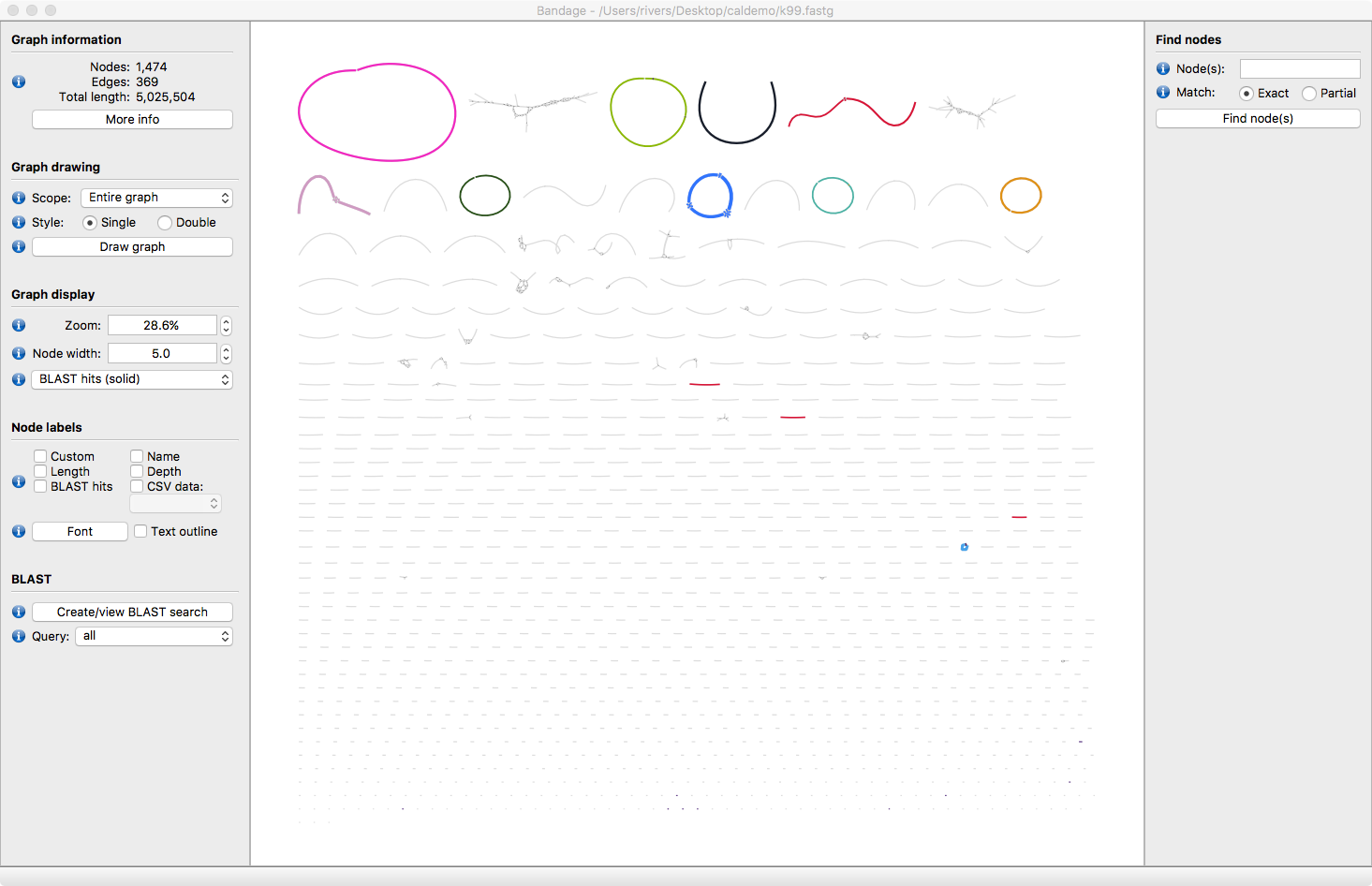
Now open Bandage and select File > Open Graph and load k99.fastg
Hit the Draw Graph button. Now all the assembled contigs are visible. Some are circular, some are linear and some have bubbles in the assembly.
IF you have a Ssand-alone copy of Blast+ installed on your computer you can label the contigs with with the reference genomes.
Download the reference fasta file here: Ref_database.fna : Download
Select Build blast database
Select Load from Fasta File and load Ref_database.fna
Select Run Blast Search then Close
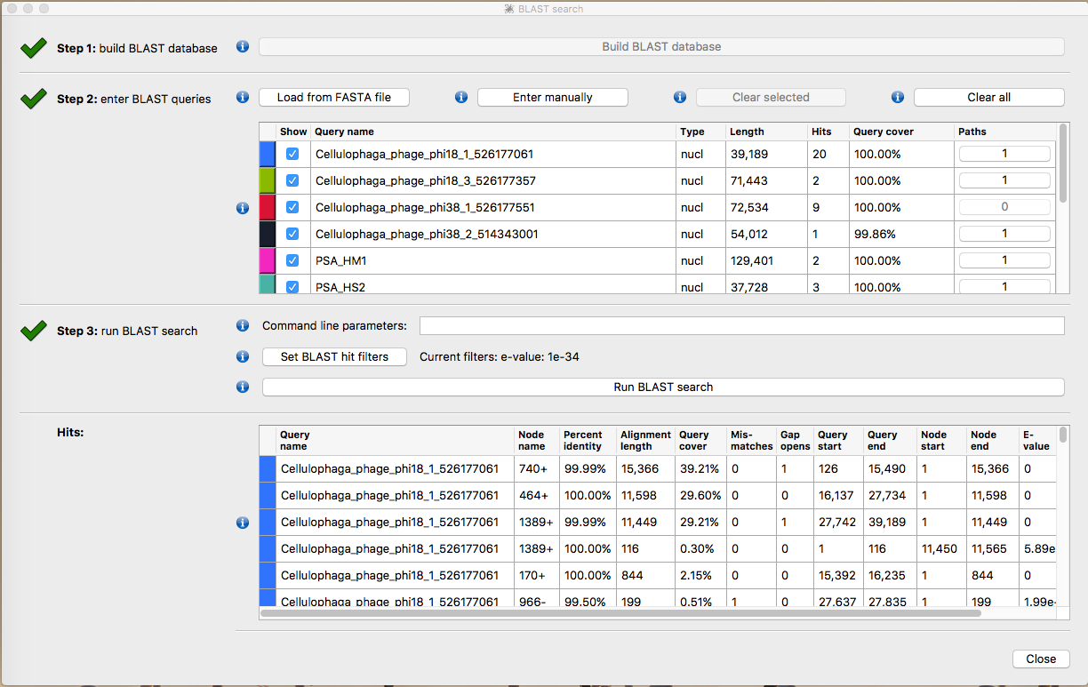
The contigs will now be taxonomically annotated. Take some time to explore the structure of the contigs. Which ones look correct? What kinds or errors are present in the assembly?
What are the contigs that assembled but were not identified by Blasting to our reference database? The fourth largest node ,Node 987 is actually genomic DNA from the bacteria Cellulophaga baltica the host of the 6 of the phages in our metagenome. Our protocol can detect and assemble this host DNA even though its present at 10-100 times lower abundance than the phages in our sample.
If we go back to the Ceres command line we can continue with the next common step in read based assembly, mapping. Two common types of mapping can occur. You can map reads back to a known reference. This is great if you have closely related organisms of interest and you are trying to understand population variance or quantify known organisms. A number of programs can be used for mapping. Bowtie2 is the most common but in this case we will use bbmap.
Map reads back to known reference
bbmap.sh \
  ref=/project/microbiome_workshop/metagenome/viral/data/Ref_database.fna \
  in=data/10142.1.149555.ATGTC.subset_500k.trimmed.fastq.gz \
  out=data/10142.1.149555.ATGTC.map_to_genomes.sam \
  nodisk \
  usejni=t \
  pigz=t \
  threads=40 \
  bamscript=bamscript1.sh
Time to run: 1 minute
When the results are mapped to a reference we are able to infer the Error rate for insertions, substitutions and deletions in our sequences. Almost all of these errors come from sequencing itself, not assembly. Note too, how much higher the error rate is for Read 2 than Read 1.
We can also see the insert size for those reads that did not merge is 300.
   ------------------   Results   ------------------

Genome:                	1
Key Length:            	13
Max Indel:             	16000
Minimum Score Ratio:  	0.56
Mapping Mode:         	normal
Reads Used:           	496904	(73428502 bases)

Mapping:          	303.347 seconds.
Reads/sec:       	1638.07
kBases/sec:      	242.06


Pairing data:   	pct reads	num reads 	pct bases	   num bases

mated pairs:     	 47.1367% 	   117112 	 47.5180% 	    34891788
bad pairs:       	  0.1139% 	      283 	  0.1111% 	       81554
insert size avg: 	  300.37


Read 1 data:      	pct reads	num reads 	pct bases	   num bases

mapped:          	 47.7621% 	   118666 	 47.7346% 	    17650903
unambiguous:     	 47.7497% 	   118635 	 47.7229% 	    17646580
ambiguous:       	  0.0125% 	       31 	  0.0117% 	        4323
low-Q discards:  	  0.0000% 	        0 	  0.0000% 	           0

perfect best site:	 43.3645% 	   107740 	 43.4335% 	    16060475
semiperfect site:	 43.4748% 	   108014 	 43.5444% 	    16101468
rescued:         	  3.1821% 	     7906

Match Rate:      	      NA 	       NA 	 99.4266% 	    17612450
Error Rate:      	  8.9689% 	    10643 	  0.4979% 	       88197
Sub Rate:        	  8.3891% 	     9955 	  0.1328% 	       23519
Del Rate:        	  0.2284% 	      271 	  0.3563% 	       63115
Ins Rate:        	  0.6143% 	      729 	  0.0088% 	        1563
N Rate:          	  0.2958% 	      351 	  0.0755% 	       13371


Read 2 data:      	pct reads	num reads 	pct bases	   num bases

mapped:          	 47.3202% 	   117568 	 47.4124% 	    17282474
unambiguous:     	 47.3057% 	   117532 	 47.4002% 	    17278009
ambiguous:       	  0.0145% 	       36 	  0.0122% 	        4465
low-Q discards:  	  0.0000% 	        0 	  0.0000% 	           0

perfect best site:	  1.3971% 	     3471 	  1.3724% 	      500267
semiperfect site:	  1.4486% 	     3599 	  1.4246% 	      519288
rescued:         	  0.4162% 	     1034

Match Rate:      	      NA 	       NA 	 91.5571% 	    16625718
Error Rate:      	 96.8691% 	   113888 	  8.3635% 	     1518716
Sub Rate:        	 95.1773% 	   111899 	  3.3643% 	      610918
Del Rate:        	  7.0826% 	     8327 	  4.8262% 	      876386
Ins Rate:        	  7.7478% 	     9109 	  0.1730% 	       31412
N Rate:          	  0.2705% 	      318 	  0.0794% 	       14426
The mapper writes text-based sam mapping files. It’s usually helpful to convert these files to a binary format called bam which is faster to access and smaller. Fortunately, bbmap will automatically make a little script to do that for us using the program Samtools. To run it enter this command.
./bamscript1.sh
It is also possible to map reads back to the contigs we just generated. Reads are mapped back to contigs for several reasons. Once genes are called gene counts can be derived from mapping data. Contig mapping data is also used in genome binning.
Map reads back to known reference
bbmap.sh \
  ref=data/megahit/final.contigs.fa \
  in=data/10142.1.149555.ATGTC.subset_500k.trimmed.fastq.gz \
  out=data/10142.1.149555.ATGTC.map_to_contigs.sam \
  nodisk \
  usejni=t \
  pigz=t \
  threads=40 \
  bamscript=bamscript2.sh
Time to run: 1 minute
With the contigs the match-rate was much higher. 95% of our reads map back to the assembly which is a very high number. in a well assembled complex metagenome we might expect 50-70% of reads to map.
Pairing data:   	pct reads	num reads 	pct bases	   num bases

mated pairs:     	 97.0034% 	   241007 	 97.8497% 	    71849602
bad pairs:       	  1.1938% 	     2966 	  1.1811% 	      867288
insert size avg: 	  298.83


Read 1 data:      	pct reads	num reads 	pct bases	   num bases

mapped:          	 99.1592% 	   246363 	 99.1688% 	    36669800
unambiguous:     	 99.1447% 	   246327 	 99.1548% 	    36664611
ambiguous:       	  0.0145% 	       36 	  0.0140% 	        5189
low-Q discards:  	  0.0000% 	        0 	  0.0000% 	           0

perfect best site:	 90.2730% 	   224285 	 90.4738% 	    33454627
semiperfect site:	 90.7552% 	   225483 	 90.9576% 	    33633528
rescued:         	  6.4733% 	    16083

Match Rate:      	      NA 	       NA 	 99.6846% 	    36578005
Error Rate:      	  8.4838% 	    20901 	  0.2057% 	       75478
Sub Rate:        	  8.3377% 	    20541 	  0.1334% 	       48939
Del Rate:        	  0.2322% 	      572 	  0.0653% 	       23946
Ins Rate:        	  0.1510% 	      372 	  0.0071% 	        2593
N Rate:          	  0.5707% 	     1406 	  0.1097% 	       40263


Read 2 data:      	pct reads	num reads 	pct bases	   num bases

mapped:          	 98.3647% 	   244389 	 98.8024% 	    36014811
unambiguous:     	 98.3172% 	   244271 	 98.7783% 	    36006044
ambiguous:       	  0.0475% 	      118 	  0.0241% 	        8767
low-Q discards:  	  0.0000% 	        0 	  0.0000% 	           0

perfect best site:	  2.2169% 	     5508 	  2.1948% 	      800050
semiperfect site:	  2.7184% 	     6754 	  2.7038% 	      985554
rescued:         	  0.7281% 	     1809

Match Rate:      	      NA 	       NA 	 93.5482% 	    34615871
Error Rate:      	 97.2331% 	   237627 	  6.3295% 	     2342103
Sub Rate:        	 95.5955% 	   233625 	  3.4830% 	     1288809
Del Rate:        	  7.0224% 	    17162 	  2.6712% 	      988449
Ins Rate:        	  7.3506% 	    17964 	  0.1752% 	       64845
N Rate:          	  0.8519% 	     2082 	  0.1224% 	       45286
As we did before we will convert the sam file to a bam file.
./bamscript2.sh
Part one of the metagenome assembly tutorial deals with the most of the heavy computational work that requires computers with high memory and many processors. In real applications this kind of work would be submitted as a batch job using the SLURM scheduler so that it can run without your being logged into Ceres.
The next major part of an assembly based workflow involves calling genes, annotating genes and binning contigs into genomes. We will address this in Part 2 of the metagenomics tutorial.